Modeling

This section covers modeling completing data query part and pre-modeling. We will reach out models fitting and ensembling

Model fitting

Model fitting is the ability we give to a machine to generalize data on which the model is trained. In practice, it consists of provide training data and some parameters to models in a way that can approach the test data the model don’t see yet. See this section to learn more about data partition into training and test data.

Firstly, select the models that you plan to use. We recommend selecting multiple models and fit them to check which provide the best performance. The choice of model is done in pre-modeling part of nimo clicking on button. In the modal that appears, click in the algorithm field to choose the model(s) you want to perform.

For example purpose, we select Random Forest (RF), Support Vector Machine (SVM) and Generalized Linear Models (GLM) algorithm. Then click on Ok button to close the modal. This is required if you exit the app after select the algorithm(s) and set up a working directory. Except that you don’t need to define a working directory again. The interface for model fitting appear now in Fitting menu of nimo app.

Interface for species distribution model fitting in nimo

You need the input data. If a break was taken until Extraction and data stemming from was saved in local, you must import it checking ‘Use existing data’ check box. If no, the data got from extraction will automatically integrated. For example purpose, we import data previously processed and available here. After import data, an option relevant to Ensemble of Small Models (ESM) appears to let decide if it is standard model that will be fitted or ESM model.

Our occurrence data is poor, although for many years (from 2016 to 2022). The sample size is limited to 25 records. So we prefer fit an Ensemble Small Models, checking ESM option. This switches model fitting fields from standard to ESM.

Ensemble Small Models fitting interface using Support Vector Machine (SVM) and Generalized Linear Models (GLM) algorithm in nimo

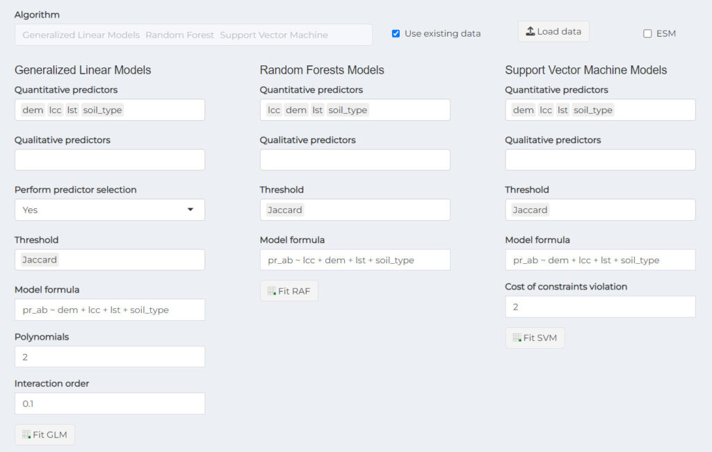
As you can remark, Random forest field disappear. This algorithm is not available for ESM. In case predictors don’t appear for selection, uncheck and check ‘Use existing data’ check box. Now let’s move on to explain some of the common and distinct parameters of these two models

Quantitative predictors: column names of quantitative predictor variables. This can only construct models with continuous variables and does not allow categorical variables.

Threshold: used to get binary suitability values (i.e. 0,1). It is useful for threshold-dependent performance metrics. It is possible to use more than one threshold type. All threshold available are used if any threshold is provided explicitly. The following threshold criteria are available:

Sensitivity = specificity: Threshold at which the sensitivity and specificity are equal.
TSS: Threshold at which the sum of the sensitivity and specificity is the highest (also known as threshold that maximizes the TSS).
Jaccard : The threshold at which Jaccard is the highest.
Sorensen: The threshold at which Sorensen is highest.
FPB: The threshold at which FPB (F-measure on Presence-Background data) is highest.
Sensitivity: Threshold based on a specified sensitivity value.

Polynomials – GLM: If used with values >= 2 model will use polynomials for those continuous variables (i.e. used in predictors argument). The fact that ESM are constructed with few occurrences, polynomials can cause overfitting.

Interaction order – GLM: The interaction order between explanatory variables. Default is 0. Because ESM are constructed with few occurrences it is recommended not to use interaction terms.

Cost of constraints violation – SVM: Cost of constraints violation, the ‘C’ constant of the regularization term in the Lagrange formulation.

Each model has Fit … at bottom to run fitting. Those button launch a modal that shows the modal output, like Model’s summary, Performance metric and Predicted suitability.

🔄All process above are same to fit standard models, except some additional parameters.

Small Model summaries

We provide an example interpretation of models output

The models consider different combinations of predictor variables, including Land Surface Temperature (lst), Digital Elevation Model (dem), Soil Type (soil_type), and Land Cover Classification (lcc). These models aim to understand how these environmental variables influence the presence or absence of Aardvarks. Here’s an interpretation of the output:

This result indicates the relationships between the predictor variables and the probability of Aardvark presence in Pendjari National Park. The coefficients tell you how each predictor variable contributes to the model’s prediction, and the AIC values can be used for model selection and comparison (lower AIC is generally preferred, here AIC = 70.79).

Model Overview:

The logistic regression model is used to predict the probability of Aardvark presence (binomial response variable) based on predictor variables.
The family is set to “binomial,” indicating that it’s a logistic regression model suitable for binary response variables.

Coefficients:

Intercept: The intercept term is approximately 28.04. This represents the estimated log-odds of Aardvark presence when all predictor variables are zero.
dem (Digital Elevation Model): The coefficient for dem is approximately -0.2474. This suggests that as the Digital Elevation Model (dem) increases by one unit, the log-odds of Aardvark presence decreases by approximately 0.2474 units.
lcc (Land Cover Classification): The coefficient for lcc is approximately -0.263. This indicates that as the Land Cover Classification (lcc) increases by one unit, the log-odds of Aardvark presence decreases by approximately 0.263 units.
I(dem^2) and I(lcc^2): These are quadratic terms representing the squared values of dem and lcc. They are used to capture potential nonlinear relationships.
The coefficient for I(dem^2) is approximately 0.0005028. This suggests that as the square of dem increases by one unit, the log-odds of Aardvark presence increases by approximately 0.0005028 units.
The coefficient for I(lcc^2) is approximately -0.0009647. This suggests that as the square of lcc increases by one unit, the log-odds of Aardvark presence decreases by approximately 0.0009647 units.
dem:lcc (Interaction Term): The coefficient for dem:lcc is approximately 0.0016423. This represents the interaction between dem and lcc. It indicates how the combined effect of dem and lcc influences the log-odds of Aardvark presence. In this case, an increase in the interaction term leads to an increase in the log-odds.

Model Summary:

SVM Type: C-svc (classification), indicating that this SVM model is used for classification tasks.
Parameter: Cost C is set to 2. This parameter controls the trade-off between maximizing the margin between classes and minimizing classification errors. A higher C allows for more classification errors but narrower margins.

Kernel Function: The model uses a Gaussian Radial Basis kernel function. This kernel is commonly used in SVMs for handling nonlinear relationships between predictors and the response variable.

Hyperparameter: The hyperparameter sigma is approximately 1.10104645815039. In the context of the Gaussian Radial Basis kernel, sigma determines the width of the kernel and influences the flexibility of the decision boundary. Higher values of sigma result in smoother decision boundaries.

Support Vectors: The model has identified 44 Support Vectors. Support Vectors are the data points that are most influential in determining the position of the decision boundary. These are the data points closest to the boundary between the classes.

Objective Function Value: The objective function value is -59.5716. This value represents the optimization objective of the SVM, and a lower value indicates that the SVM has successfully separated the classes with a good margin.

Training Error: The training error rate is 0.22, which means that the SVM model misclassifies approximately 22% of the training data. This indicates the model’s accuracy on the training dataset.

Standard models fitting

In this section, we will discover how to fit standard models and ensemble them. The algorithms used in Ensemble Small Models previously are renews. Proceed to algorithms selection. Be sure ESM option is unchecked in fitting menu because we don’t want fit ESM here.

The output is similar to previous model’s summaries. For GLM, If you select Yes to perform predictor selection, predictors will be selected based on backward step-wise approach. The selected predictors are represented by the model with lower AIC, indicating that this model provides a reasonably good fit to the data. Look the explanation results of the Random Forest classification model used for species distribution modeling of Aardvarks in Pendjari National Park in pane below.

Model Summary:

Model Type: Random Forest for classification. Random Forest is an ensemble machine learning technique that builds multiple decision trees and combines their predictions to make a final classification decision.
Number of Trees: The model was built with 500 decision trees.
Number of Variables Tried at Each Split: During the construction of each decision tree, only 2 randomly selected variables (predictors) were considered at each split. This parameter controls the randomness and diversity of the trees in the forest.

Out-of-Bag (OOB) Error Estimate: The OOB estimate of the error rate is 40%. This is an estimate of how well the model is expected to perform on unseen data. In this case, the model is estimated to make incorrect predictions for 40% of the data points it has not seen during training.

Confusion Matrix: The confusion matrix provides a breakdown of the model’s predictions versus the actual class labels. In this case, the classes are represented as “0” and “1,” where “0” may represent Aardvarks’ absence, and “1” may represent Aardvarks’ presence. The confusion matrix is as follows:

	Predicted 0	Predicted 1	Class error
Real 0	14	11	0.44
Real 1	9	16	0.36

In the confusion matrix:

“14” represents the number of true negatives (actual class 0 correctly predicted as 0).
“11” represents the number of false positives (actual class 0 incorrectly predicted as 1).
“9” represents the number of false negatives (actual class 1 incorrectly predicted as 0).
“16” represents the number of true positives (actual class 1 correctly predicted as 1).
“Class Error” indicates the error rate for each class. For class 0, the error rate is 0.44, and for class 1, the error rate is 0.36.

The model’s performance can be further evaluated and tuned to improve its accuracy and generalizability. Additionally, the choice of the quality of the predictor variables can significantly impact model performance.

Ensemble models

Ensemble techniques are methods that combine the predictions of multiple individual models (often called base models or weak learners) to improve overall predictive performance. The key idea behind ensemble methods is to harness the collective intelligence of multiple models to make more accurate and robust predictions than any individual model could achieve on its own. To ensemble models in nimo, go in Ensemble menu.

The models we just fit are listed. We can select Support Vector Machine (SVM) and Generalized Linear Models (GLM) and it. The resulted model can be used for prediction, as we will see in post-modeling.