Pre-modeling
The pre-modeling step in species distribution modeling refers to the preparatory phase before constructing the actual model. It involves a series of tasks aimed at gathering and preparing the necessary data, as well as conducting exploratory analyses to ensure the data is suitable for modeling. Let’s move to pre-modeling in nimo that contains five main parts.

1. Directory Setup
To start a project, you need to create a project directory, which is a folder that contains all the data and results related to your project. The project directory should have subfolders for different types of files, such as inputs, outputs, projections, calibration areas, algorithms, ensembles, and thresholds. You can use the ‘Set Directory‘ button to create these subfolders automatically, based on the options you choose. Before, you need to create a main directory, which is the folder where the project directory will be located. You can choose any location on your computer for the main directory.

Provide that folder, browsing after clicking on ‘Directory‘ in modal. You need to specify which subfolders you want to include in the project directory. For example, if you want to include calibration areas, you need to keep calibration area checked. In algorithm field, you choose algorithm(s) you plan to use for your study such as Generalized Additive Models, Maximum Entropy, Neural Networks, Generalized Linear Models, Gaussian Process, Generalized Boosted Regression, Random Forest, and Support Vector Machine.
To illustrate directory setup, suppose we created a folder called Try in a main directory labeled D:. . The algorithms chosen are Random Forest (raf) and Support Vector Machine (svm). The calibration area is checked as by default and models assemblage method used is mean (average as default). Once you action on ![]() button, you will get this tree detailed in Try folder.
button, you will get this tree detailed in Try folder.
- Inputs:
- 1_Occurrences: This directory likely contains data related to occurrences of the species that are being modeled.
- 2_Predictors: Data used as environmental predictors for the SDM.
- 1_Current: Current environmental predictor data.
- 2_Projection: Environmental predictor data for future projections.
- proj: Specific projection data.
- Outputs:
- 0_Model_performance: This directory is likely for storing the evaluation results of model performance metrics.
- 1_Current: Outputs related to the current modeling scenario.
- Algorithm: Different modeling algorithms used for current scenarios.
- raf: Outputs related to a modeling algorithm (e.g., Random Forest).
- 1_con: Outputs related to continuous predictions using the Random Forest algorithm.
- 2_bin: Outputs related to binary predictions using the Random Forest algorithm.
- svm: Outputs related to another modeling algorithm (e.g., Support Vector Machine).
- 1_con: Outputs related to continuous predictions using the SVM algorithm.
- 2_bin: Outputs related to binary predictions using the SVM algorithm.
- raf: Outputs related to a modeling algorithm (e.g., Random Forest).
- Ensemble: Outputs related to ensemble model predictions for the current scenario.
- mean: Outputs related to ensemble predictions taking the mean of two models.
- 1_con: Outputs related to continuous ensemble predictions using the mean.
- 2_bin: Outputs related to binary ensemble predictions using the mean.
- mean: Outputs related to ensemble predictions taking the mean of two models.
- 2_Projection: Outputs related to projections (future scenarios).
- proj: Specific projection outputs.
- Algorithm: Different modeling algorithms used for projections.
- raf: Outputs related to a modeling algorithm (e.g., Random Forest) for projections.
- 1_con: Outputs related to continuous predictions using the Random Forest algorithm for projections.
- 2_bin: Outputs related to binary predictions using the Random Forest algorithm for projections.
- svm: Outputs related to another modeling algorithm (e.g., Support Vector Machine) for projections.
- 1_con: Outputs related to continuous predictions using the SVM algorithm for projections.
- 2_bin: Outputs related to binary predictions using the SVM algorithm for projections.
- raf: Outputs related to a modeling algorithm (e.g., Random Forest) for projections.
- Ensemble: Outputs related to ensemble model predictions for projections.
- mean: Outputs related to ensemble predictions for projections, using the mean.
- 1_con: Outputs related to continuous ensemble predictions using the mean for projections.
- 2_bin: Outputs related to binary ensemble predictions using the mean for projections.
- 1_con: Outputs related to continuous ensemble predictions using the mean for projections.
- mean: Outputs related to ensemble predictions for projections, using the mean.
- Algorithm: Different modeling algorithms used for projections.
- proj: Specific projection outputs.
- Algorithm: Different modeling algorithms used for current scenarios.
This directory structure is designed to organize various inputs, modeling algorithms, ensemble methods, and outputs for species distribution modeling. It distinguishes between current and projected scenarios and provides a clear structure for different algorithms and ensemble techniques. The actual content and purpose of the directories may vary depending on the specific context or study.
2. Calibration area
Calibration area is the geographic region where the environmental data and the occurrence records of a species are used to train a SDM (Machado-Stredel et al., 2021). The calibration area, or geographic space used to train species distribution models, is an important consideration that impacts several aspects of modeling. It determines from where pseudo-absence and background data are sampled to train the model. It also affects the model evaluation metrics and the spatial patterns of predicted habitat suitability (Velazco et al., 2022). Four methods are implemented to calibrate the species distribution area.
Before apply any method, provide the occurrence data by checking ‘import data‘ and load data in .csv or .txt file format. The modal that appears let you characterize the data.
- Species column : Select the column that contains species name in the dataset
- Species : Select species of interest. If you select more than one, nimo considers as one species. You select many species if there are similar.
- Longitude and Latitude: column in dataset that represents longitude and latitude respectively.
- Variable to conserve: Other variables to consider, such as habitat type. The most GBIF data has incomplete information for habitat field.

Once the inputs are provided according to research or study, Valid dataset, clicking on button. Without error, the species occurrence data appears in ‘Unique Occurrence’ tab. The duplicated data appears in ‘Duplicated Occurrence’. Those data will be ignored in suite of the modeling process.
In ‘Geographic’ tab, you will be able to set the calibration area. Area calibration requires occurrence data. Be sure the data is provided, and their geographic distribution is correctly display. Click ‘Add layer‘ button to add an existing geographic vector Esri Shapefile (.shp) or Keyhole Markup Language (.kml) format that represents the delimitation of the area of interest. Then click ‘Calibrate area‘. In modal, choose a suitable basing on area calibration methods explained below.
| Method | Description | Parameter | Output |
| Buffer | Calibration area is defined using buffers around presence points. Users can specify the distance around points using the “width” argument. | Width interpreted in m if the CRS has a longitude/latitude, or in map units in other cases. |  |
| Buffered minimum convex polygon | Like Minimum convex polygon, this method produces a simpler shape surrounding the outlier presence points adding distance around points using the “width” argument. |  | |
| Buffered minimum convex polygon | The method produces a simpler shape surrounding the outlier presence points. More the points are dispersed in area, more the area calibrated is big. | – |  |
| Mask | Calibration area is defined by selected polygons in a spatial vector intersected by presence point. This is useful if user expects species distributions to be associated with ecologically significant (and mapped) ecoregions, or are interested in distributions within political boundaries | The “Filter by” is with the column name from spatial vector used for filtering polygons. |  |
The last validation of area calibration is taken in account for the rest of modeling procedure.
3. Predictors
In species distribution modeling, predictors are variables or factors that are used to predict the distribution of species. These predictors can be environmental variables such as temperature, precipitation, elevation, soil type/moisture, land cover, etc. They can also include human-related variables such as proximity to roads, urban areas, or other human activities. The idea behind using predictors is to identify the environmental conditions or factors that are associated with the presence or absence of a species in a given area.
However, two or more predictors are correlated with each other – collinearity. This can cause problems in the modeling process because it violates the assumption of independence among predictors and can lead to unstable or unreliable model results.

3.1. Reducing collinearity
When collinearity exists, it becomes difficult to determine the unique contribution of each predictor to the model. To address collinearity, several approaches can be employed. One common approach is to assess the correlation matrix among predictors and remove highly correlated variables from the model.
Come into flexsdm R package, nimo’s user can reduce collinearity using four methods. These methods serve as supplementary tools that can assist in the predictor selection. However, it is important to note that predictor selection is a complex task and should primarily be based on the understanding of the relationship between the environment and the biology of the species in question. The methods offer options for exploring the relationships between predictor variables, but they should be used in conjunction with ecological knowledge and careful consideration of the species’ ecological requirements.
Pearson correlation
This method calculates the Pearson correlation coefficient between each pair of environmental variables. It returns the environmental variables that have a correlation below a given threshold (default is 0.7). It also provides the names of the variables that had a correlation above the threshold and were removed, as well as a correlation matrix of all the environmental variables.
Variance inflation factor
This method calculates the variance inflation factor (VIF) for each predictor variable. The VIF measures how much the variance of a regression coefficient is increased due to multicollinearity. Predictors with a VIF higher than the chosen threshold (default is 10) are removed. The output of this method is similar to the Pearson correlation method, including a the retained variables, a list of removed variables, and a correlation matrix.
Principal component analysis (PCA)
It identifies the principal components that account for 95% of the total variance in the system. The output includes the selected environmental variables, a matrix with the coefficients of the principal components for the predictors, and a tibble with the cumulative variance explained by the selected principal components.
Factorial analysis (FA)
This method also aims to reduce dimensionality through a factorial analysis. It selects the predictor(s) with the highest correlation to each axis. The outputs of this method are similar to the PCA method.
4. Data filtering
Occurrence data filtering is a process of removing or thinning out redundant data points from species occurrence data. This is done to reduce sample bias, which is a common issue in ecological studies. Inherit flexsdm, nimo offers two ways for filtering, based on geographical or environmental “thinning”. The points are randomly removing where they are dense (oversampling) in geographical or environmental space (Valera et al., 2014). This can improve model performance and reduce redundancy in the data to improve the accuracy of models and provide more reliable predictions.

Environmental filtering: It focuses on removing data points based on their similarity in environmental conditions. It aims to reduce redundancy in the data by retaining only a representative subset of occurrences across various environmental gradients. This method ensures that the selected data points cover a broader range of environmental conditions.
Geographical Filtering: It seeks to reduce oversampling in specific geographic regions by randomly thinning out occurrences that are densely clustered in certain areas. This approach helps balance the spatial distribution of data.
To filter occurrence data in nimo, pass through Occurrence data filtering button(![]() ) – 8th button in screenshot in predictors section above. The button brings you to this modal
) – 8th button in screenshot in predictors section above. The button brings you to this modal

Geographical filtering has three alternatives for determining the distance threshold between a pair of points:
- moran – determines the threshold as the distance between points that minimizes the spatial autocorrelation in the occurrence data;
- cellsize – filters occurrences based on the resolution of the predictors (or a specified coarser resolution);
- defined – allows the user to determine the distance threshold manually.
After chosen the filtering type and provided parameters according to desire, click ![]() . The Distribution tab shows the plot of new data and Filtered data tab shows the table of that data.
. The Distribution tab shows the plot of new data and Filtered data tab shows the table of that data.
Despite the relevance of filtering occurrence data, it remains optional, especially when the number of records is small. At this point, nimo v.0.2.0 does not integrate the filtered data directly into the pre-modelling suite. So if the filter is applied, click on the save button to export this new occurrence data. Then import again and repeat all the steps up to this level without applying the filter a second time. The next step will be the partition.
5. Partition
The data partion allows us to have training data and test data to fit and turn models. It is a crucial step in constructing Species Distribution Models (SDMs), and flexsdm offers several options for this purpose, including Random, Spatial band, Spatial block and Environmental and Spatial. Let’s delve into each of these methods:
5.1. Random – Conventional Data Partitioning Methods:
The random function enables users to split species occurrence data using conventional partitioning techniques such as k-folds, repeated k-folds, leave-one-out cross-validation, and bootstrap partitioning. For example, using the “kfold” method with 05 folds would result in 05 sets of Aardvark occurrence data, each containing 05 observations.
5.2. Spatial Band Cross-Validation:
Both Spatial band and Spatial block partition data based on their geographic spatial distribution. These methods are particularly valuable when assessing a model’s transferability to different regions or time periods. The Spatial band method assesses various numbers of spatial partitions using latitudinal or longitudinal bands and selects the most suitable number of bands based on factors like spatial autocorrelation, environmental similarity, and the distribution of presence/absence records within each band. Its output includes a table with location information and partition assignments, details about the best partition, and a plot illustrating the chosen grid.
5.3. Spatial Block Cross-Validation:
Similar to Spatial band, this method divides data into spatial blocks. However, instead of bands, it explores different raster cell sizes and identifies the one that best fits the input dataset. It divides the data into separate “blocks” for training and testing.
5.4. Environmental and Spatial Cross-Validation:
This is the final partitioning way in nimo. The method explores different numbers of environmental partitions based on the K-means clustering algorithm and selects the most suitable partition for a given dataset. It considers factors such as spatial autocorrelation, environmental similarity, and the distribution of presence and/or absence records within each partition. The partitioning is based on both environmental and spatial factors, resulting in a map illustrating the chosen partitioning scheme.
| Methods | Parameters |
| Spatial band | – Across: axis along which bands will be made across different degrees of longitude or latitude – Min bands: minimum number of spatial bands to be tested. – Max bands: maximum number of spatial bands to be tested. |
| Spatial block | – Min precision: minimum value used for multiplying raster resolution and define the finest resolution to be tested. – Max precision: maximum value used for multiplying raster resolution and define the coarsest resolution to be tested. – Number of grids: number of grid to be tested between Min precision and Max precision. |
| – Number of partitions: number of partition (subset) – Min occurrence: minimum number of presences or absences in a partition fold. The value should be based on the number of predictors to avoid over-fitting or error when fitting models for a given fold. – Proportion: proportion of points used for testing autocorrelation between groups. | |
To apply or take in consideration the partition method chosen, click ![]() button.
button.
6. Background/Pseudo-absence sampling
Background and pseudo-absence data sampling are two common methods used to generate data for species distribution modeling. Background data is a set of random points that are assumed to be absent of the species of interest, while pseudo-absence data is generated by selecting points from the study area that are not known to contain the species of interest. The main difference between these two methods is that background data is generated randomly, while pseudo-absence data is generated based on the study area’s characteristics.
Both background and pseudo-absence data sampling method are available in nimo. It returns a table separated in two tab, one (New points) for data generated and second (Updated occurrence) for original occurrence completed by data generated.

7. Extraction
The last step in pre-modeling phase in species distribution modeling workflow in nimo is environmental data extraction at the ‘presences + absences’/’pseudo-absences’/’background’ point locations. In Extraction menu, extraction can be done easily by clicking on ![]() . This action extracts environmental data values based on occurrence and returns a table with the original data + additional columns for the extracted environmental variables at those locations.
. This action extracts environmental data values based on occurrence and returns a table with the original data + additional columns for the extracted environmental variables at those locations.

The environmental variable used here depend on collinearity reducing applied. Only predictor not removed are available.
The output can be saved via save button. In our application example, the extracted environmental data basing on Orycteropus afer occurrence in Pendjari National Park can be accessed here.