Species distribution modeling: key concepts

These pages explain species distribution modeling (SDM) and how to carry out each step in nimo, from occurrence records to maps of habitat suitability. No programming is needed: every step is done in the nimo interface. Readers who already know SDM can go straight to the page they need.

The documentation is organised in seven pages:

1. Species distribution modeling: key concepts (this page)
2. Occurrence data
3. Pre-modeling
4. Modeling
5. Post-modeling
6. Reproducible script
7. Hands-on practice with the example data

What is a species distribution model?

A species distribution model relates where a species has been observed to the environmental conditions at those places (climate, vegetation, topography, land use, distance to water, and so on). Once that relationship is estimated, it is used to predict how suitable every location of a study area is for the species, including places where nobody has looked for it (Guisan & Thuiller 2005; Elith & Leathwick 2009).

The result is usually a map of habitat suitability, with values from 0 (unsuitable) to 1 (highly suitable), and often a binary map (suitable or unsuitable) obtained by applying a threshold to the suitability values.

SDMs are used to:

• identify areas where a rare or threatened species may occur and guide field surveys;
• prioritise areas for protection or restoration;
• assess the risk of invasion by alien species;
• explore how species distributions may change under future climate or land use;
• understand which environmental factors limit a species.

The ecological niche

SDMs rest on the concept of the ecological niche. Hutchinson (1957) defined the niche as the set of environmental conditions under which a species can maintain a population. Two views of the niche matter for modeling:

• The fundamental niche is the full range of conditions the species can tolerate physiologically.
• The realized niche is the part of the fundamental niche the species actually occupies, once competition, predation, dispersal limits and human pressure are taken into account.

Because SDMs are built from field observations, they describe the realized niche, not the fundamental one.

A useful way to picture this is the BAM framework (Soberón & Peterson 2005). A species is found where three conditions overlap:

• B (biotic): interactions with other species allow it to persist;
• A (abiotic): the environment is suitable;
• M (movement): the area has been accessible to the species through dispersal.

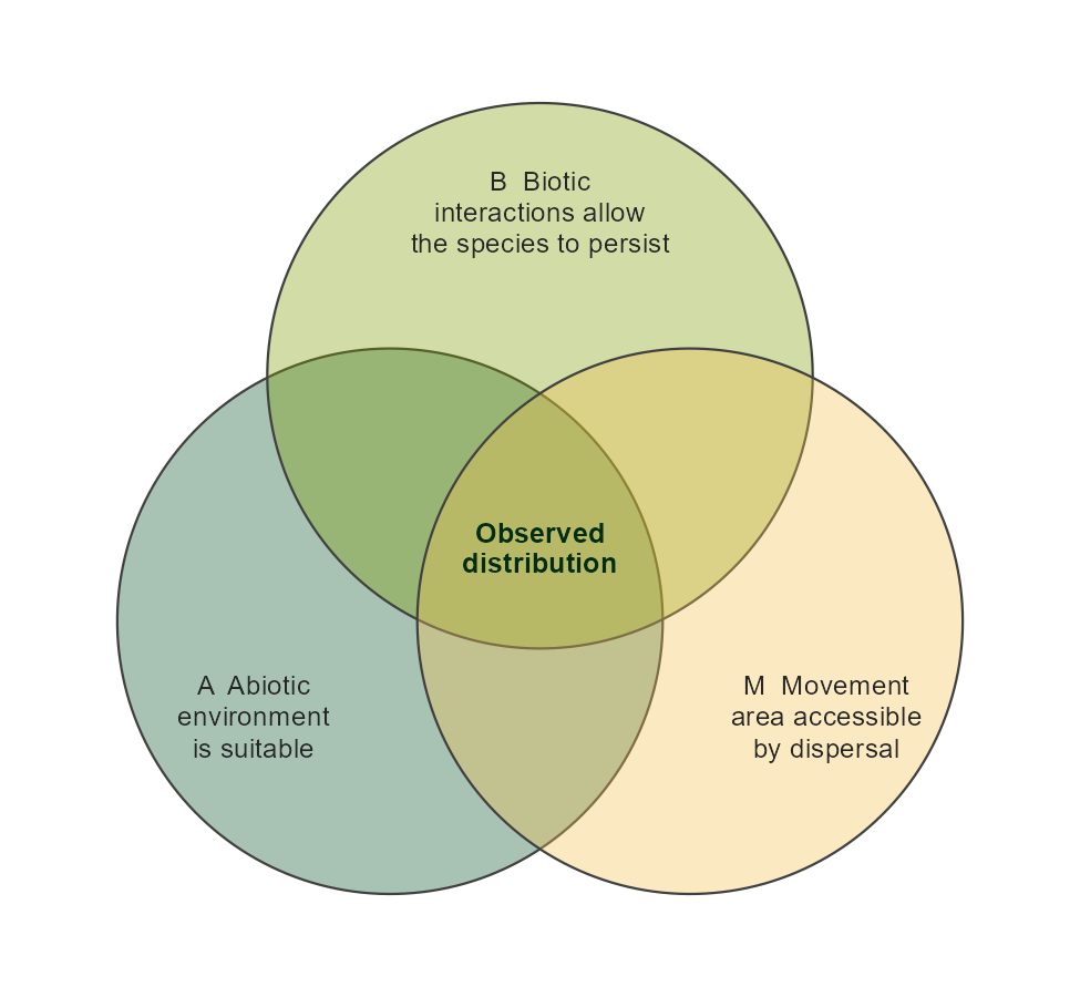
The M component explains why the choice of the study area, called the calibration area in nimo, matters so much: the model should learn from places the species could have reached.

Types of occurrence data

Models differ according to the information available about where the species is absent.

Data type	What it contains	Typical source
Presence-only	Places where the species was recorded	Museum collections, GBIF, opportunistic sightings
Presence-absence	Places where the species was recorded and places surveyed where it was not found	Systematic surveys, camera trapping, transects

Most data available online are presence-only. A model still needs to contrast presences with something, so two kinds of artificial points are generated:

• Background points describe the range of environmental conditions available in the calibration area. They do not claim the species is absent.
• Pseudo-absences are points treated as absences, usually placed away from presences in geographical or environmental space to make that assumption more plausible (Barbet-Massin et al. 2012).

nimo handles both data types. With presence-only data, the Pre-modeling part shows how to sample background points or pseudo-absences.

The modeling workflow

Every SDM follows the same broad steps. nimo organizes its menus around them.

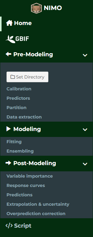
Step	Purpose	Where in nimo
Occurrence data	Gather and clean species records	GBIF, Pre-Modeling > Calibration
Calibration area	Define the region the model learns from	Pre-Modeling > Calibration
Predictors	Choose environmental layers and reduce redundancy among them	Pre-Modeling > Predictors
Data quality	Remove outliers and reduce sampling bias	Pre-Modeling > Predictors
Partition	Split records into training and testing sets	Pre-Modeling > Partition
Background or pseudo-absences	Create contrast points for presence-only data	Pre-Modeling > Partition
Extraction	Read predictor values at each record	Pre-Modeling > Data extraction
Model fitting	Fit and evaluate one or several algorithms	Modeling > Fitting
Ensemble	Combine models	Modeling > Ensembling
Interpretation	Understand what drives the predictions	Post-Modeling > Variable importance, Response curves
Prediction	Map suitability across the study area	Post-Modeling > Predictions
Reliability	Check extrapolation, uncertainty and overprediction	Post-Modeling > Extrapolation & uncertainty, Overprediction correction
Reporting	Keep the R code of the whole analysis	Script

Evaluating a model

A model is only useful if it predicts well records it has not seen. That is why the records are split into a training set, used to fit the model, and a testing set, used to measure its performance. Repeating the split several times (for example with k-fold cross-validation) gives a more reliable estimate.

Performance metrics compare predicted suitability with the observed presences and absences of the testing set:

• Threshold-independent metrics use the continuous suitability values. The most common is the AUC (area under the ROC curve): 0.5 means no better than random, 1 means perfect discrimination. The Boyce index is designed for presence-only data and measures whether presences are more frequent than expected in areas of high suitability (Hirzel et al. 2006).
• Threshold-dependent metrics first turn suitability into a binary map with a threshold, then count correct and wrong predictions. Sensitivity is the proportion of presences predicted as suitable, specificity the proportion of absences predicted as unsuitable, and the TSS (true skill statistic) equals sensitivity + specificity – 1, from -1 to 1 (Allouche et al. 2006). Kappa, Jaccard, Sorensen and FPB are other metrics of this family.

The Modeling page describes the metrics and thresholds available in nimo in more detail.

Assumptions and limits

SDMs give valuable information, but their predictions rest on assumptions worth keeping in mind:

• Equilibrium: the species occupies all suitable areas it can reach. Species that are spreading (invasive species) or recovering break this assumption.
• Representative sampling: records reflect where the species lives, not where observers go. Records are often clustered near roads, towns or research stations; this sampling bias can make the model learn the distribution of observers instead of the species. The Pre-modeling page shows how to reduce it.
• Relevant predictors: the model can only use the variables it is given. Missing a limiting factor, or including irrelevant ones, degrades predictions.
• Transferability: predictions outside the conditions seen during training (another region, or the future) are extrapolations and are less reliable. The Post-modeling page shows how to measure extrapolation.

Glossary

Term	Meaning
Absence	Location surveyed where the species was not detected
Background points	Points describing the environment available in the calibration area
Calibration area	Region used to train the model (also called accessible area, M)
Collinearity	Strong correlation between predictors
Cross-validation	Repeated splitting of records into training and testing sets
Ensemble	Combination of the predictions of several models
Extrapolation	Prediction in conditions outside those used for training
Habitat suitability	Model output from 0 to 1 expressing how favourable a location is
Predictor	Environmental variable used to explain the distribution
Presence	Location where the species was recorded
Pseudo-absence	Artificial point treated as an absence
Threshold	Suitability value used to separate suitable from unsuitable

References

• Allouche, O., Tsoar, A., & Kadmon, R. (2006). Assessing the accuracy of species distribution models: prevalence, kappa and the true skill statistic (TSS). Journal of Applied Ecology, 43, 1223-1232.
• Barbet-Massin, M., Jiguet, F., Albert, C. H., & Thuiller, W. (2012). Selecting pseudo-absences for species distribution models: how, where and how many? Methods in Ecology and Evolution, 3, 327-338.
• Elith, J., & Leathwick, J. R. (2009). Species distribution models: ecological explanation and prediction across space and time. Annual Review of Ecology, Evolution, and Systematics, 40, 677-697.
• Guisan, A., & Thuiller, W. (2005). Predicting species distribution: offering more than simple habitat models. Ecology Letters, 8, 993-1009.
• Hirzel, A. H., Le Lay, G., Helfer, V., Randin, C., & Guisan, A. (2006). Evaluating the ability of habitat suitability models to predict species presences. Ecological Modelling, 199, 142-152.
• Hutchinson, G. E. (1957). Concluding remarks. Cold Spring Harbor Symposia on Quantitative Biology, 22, 415-427.
• Soberón, J., & Peterson, A. T. (2005). Interpretation of models of fundamental ecological niches and species’ distributional areas. Biodiversity Informatics, 2, 1-10.