Modeling
With the modeling table ready (see Pre-modeling), models can be fitted, evaluated and combined. This page presents the algorithms available in nimo, their settings, how performance is measured, and how to combine models into an ensemble.
Choosing algorithms
No algorithm is best in every situation. Comparing several algorithms, and combining them, is common practice. The algorithms available in nimo belong to four families.
| Family | Algorithm | Data | Strengths | Limits |
|---|---|---|---|---|
| Envelope and distance | Bioclim | Presences (absences used for evaluation) | Simple, easy to interpret, stable with few records | Ignores absences; rectangular envelope; no interactions |
| Domain | Presences (absences used for evaluation) | Works with very few records | Sensitive to outliers; no extrapolation beyond records | |
| Regression | Generalized Linear Models (GLM) | Presences and absences or pseudo-absences | Interpretable coefficients; smooth responses | Responses limited to the chosen form (linear, quadratic) |
| Generalized Additive Models (GAM) | Presences and absences or pseudo-absences | Flexible smooth responses | Can overfit with few records | |
| Machine learning | Random Forest | Presences and absences or pseudo-absences | Captures interactions and complex responses | Less interpretable; can overfit |
| Generalized Boosted Regression (GBM) | Presences and absences or pseudo-absences | High predictive performance | Several settings to tune | |
| Support Vector Machine (SVM) | Presences and absences or pseudo-absences | Handles complex boundaries | Less interpretable | |
| Neural Networks | Presences and absences or pseudo-absences | Very flexible | Needs many records; less interpretable | |
| Gaussian Process | Presences and absences or pseudo-absences | Smooth, flexible responses | Slow with many records | |
| Maximum entropy | Maxent | Presences and background points | Designed for presence-background data; widely used | Several settings to tune |
Bioclim
Bioclim (Busby 1991; Booth et al. 2014) describes the environmental envelope of the species from its presences. For each predictor, the value of a location is compared to the values observed at presences: values near the median score close to 1, values at the edge of the observed range score close to 0, and values outside the range score 0. The scores of the predictors are then combined into one suitability value.
nimo offers two settings:
- Limiting tails: whether both low and high values of the predictors limit suitability (classic Bioclim), only low values, or only high values. For example, for a variable such as vegetation cover, only low values may limit a forest species.
- Combine variables with:
- Minimum (classic Bioclim): the most limiting variable sets suitability;
- Geometric mean: still 0 outside the range of any variable, but less dominated by a single variable;
- Arithmetic mean: the most permissive combination.
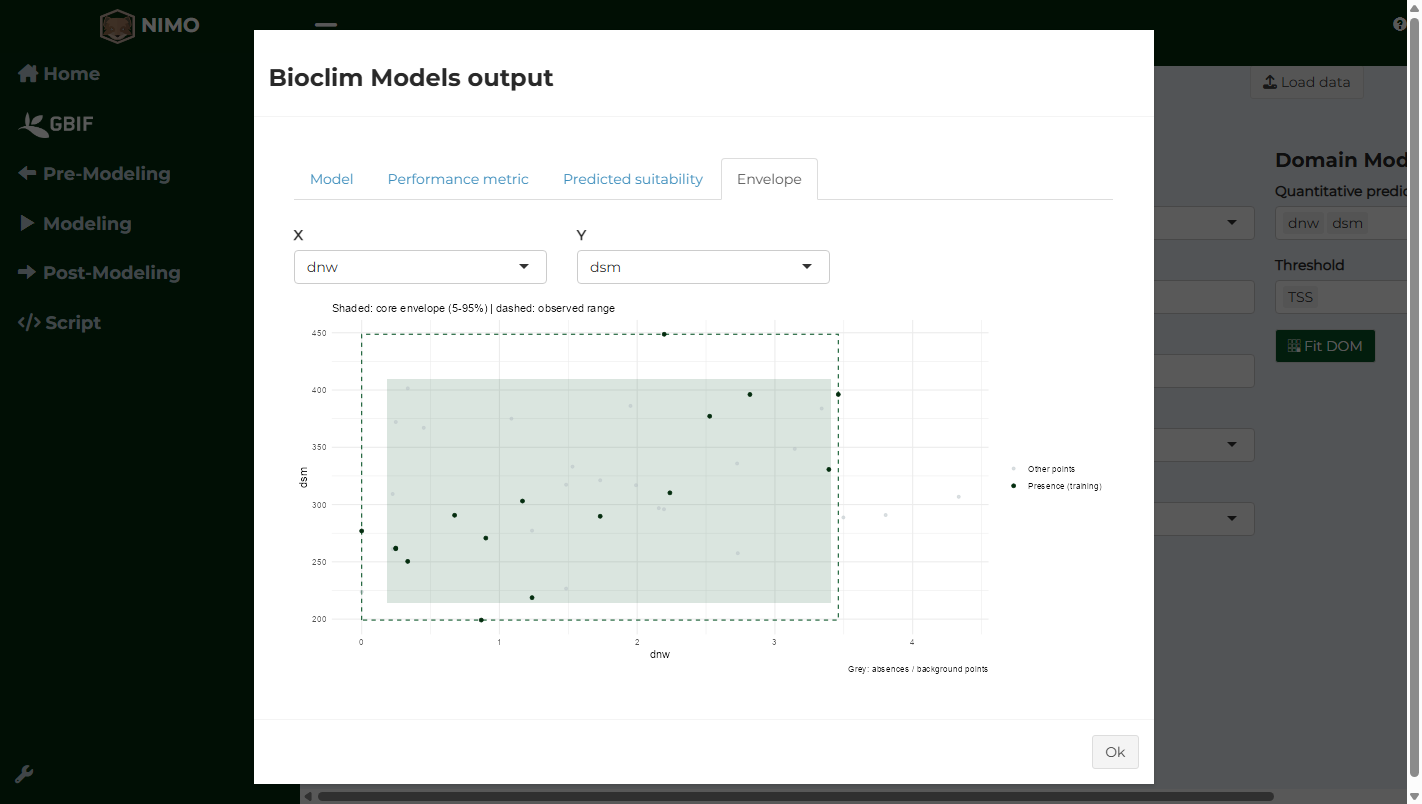
After fitting, the Envelope tab plots the presences in the space of two predictors, with the core envelope (5th to 95th percentiles, shaded) and the observed range (dashed). Grey points are absences or background points.
Domain
Domain (Carpenter et al. 1993) measures how similar each location is to the most similar presence, using an environmental (Gower) distance. Suitability decreases as the distance to the closest presence increases. It is useful for species with very few records.
Selecting the algorithms
The algorithms are chosen when the project directory is set (Pre-Modeling > Set Directory, field Algorithm). They then appear in Modeling > Fitting.

The fitting page
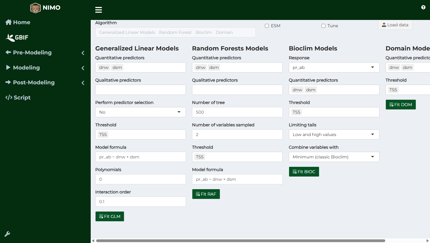
The modeling table produced by the extraction step is used automatically. A table saved earlier can be used instead with Load data.
At the top of the page:
- ESM switches to Ensembles of Small Models, designed for species with few records (see the post Ensemble of Small Models for species distribution modeling);
- Tune switches to hyperparameter tuning (see below).
Settings shared by all algorithms
- Quantitative predictors: continuous variables (temperature, elevation…).
- Qualitative predictors: categorical variables (soil type, land cover class…). Not available for Bioclim and Domain.
- Threshold: the method used to turn suitability into suitable or unsuitable, used to compute threshold-dependent metrics and binary maps. Several can be selected. The choice of threshold depends on the purpose of the map (Liu et al. 2005). To avoid missing occupied areas (for a threatened species), prefer No omission or a high Sensitivity. To balance errors, TSS or Sensitivity = specificity are common choices.
- No omission: the highest threshold at which all presences are predicted suitable;
- Sensitivity = specificity: the threshold at which sensitivity and specificity are equal;
- TSS: the threshold that maximizes sensitivity + specificity;
- Jaccard and Sorensen: the thresholds that maximize these similarity indices;
- FPB: the threshold that maximizes the F-measure for presence-background data;
- Sensitivity: the threshold giving a chosen sensitivity (for example 0.9, meaning 90% of presences predicted suitable).
- Model formula: for regression and some machine learning algorithms, the formula linking presence to predictors is written automatically and can be edited.
Algorithm-specific settings
| Algorithm | Setting | Meaning |
|---|---|---|
| GLM | Perform predictor selection | Keep the combination of predictors with the lowest AIC (stepwise) |
| Polynomials | Add squared (2) or higher terms to allow curved responses | |
| Interaction order | Allow combined effects of predictors | |
| GAM | Basis dimension | Flexibility of the smooth curves |
| GBM | Number of trees, Learning rate | More trees with a smaller learning rate give smoother, more stable models |
| Maxent | Classes | Feature types: linear, quadratic, hinge, product, threshold |
| Regularization | Penalty against complexity; higher values give simpler models | |
| Clamp, Type of response | Restrict predictions to the training range; output scale (cloglog is the usual choice) | |
| Neural Networks | Number of units, Weight decay | Size of the hidden layer and its penalty |
| Random Forest | Number of tree, Number of variables sampled | Trees in the forest and predictors tested at each split |
| SVM | Cost of constraints violation | Trade-off between a smooth boundary and fewer training errors |
| Bioclim | Response, Limiting tails, Combine variables with | See above |
Each algorithm has a Fit button. The window that opens shows:
- Model: the fitted model (coefficients for GLM, structure for machine learning models, envelope summary for Bioclim);
- Performance metric: performance averaged over the test folds;
- Predicted suitability: the suitability predicted for every test record, used to build ensembles;
- Envelope (Bioclim only).
Reading the performance table
Each metric is computed on the testing folds and given as a mean and standard deviation across folds. A large standard deviation means performance varies a lot depending on the records used.
| Metric | Range | Meaning |
|---|---|---|
| AUC | 0 to 1 | Probability that a random presence has higher suitability than a random absence. 0.5 = random, above 0.8 = good |
| Boyce | -1 to 1 | Whether presences are more frequent than expected where suitability is high. Suited to presence-only data |
| TSS | -1 to 1 | Sensitivity + specificity – 1 at the threshold. 0 = random, above 0.5 = good |
| Kappa | -1 to 1 | Agreement between predicted and observed classes beyond chance |
| Sensitivity (TPR) | 0 to 1 | Share of presences predicted suitable |
| Specificity (TNR) | 0 to 1 | Share of absences predicted unsuitable |
| Omission rate (OR) | 0 to 1 | Share of presences predicted unsuitable (1 – sensitivity) |
| Jaccard, Sorensen, FPB | 0 to 1 (FPB 0 to 2) | Overlap between predicted suitable area and presences |
| IMAE | 0 to 1 | Inverse mean absolute error between suitability and observations |
These thresholds of “good” performance are indicative. Compare algorithms on the same partition, and remember that performance measured with a random partition is usually higher than with a spatial partition (see Pre-modeling).
Download saves the performance table.
Tuning hyperparameters
Hyperparameters are settings fixed before fitting (number of trees, regularization, and so on). Default values do not suit every dataset. Tuning fits the model for every combination of the values you provide and keeps the combination with the best performance on the testing folds.
Tick Tune, then type several values separated by commas in the fields of the algorithm (for example Number of trees 100, 500, 1000 and Learning rate 0.01, 0.1), choose the Metric used to select the best combination, and click the tuning button of the algorithm (Tune GBM, Tune RAF, …). Tuning is available for GBM, Maxent, Neural Networks, Random Forest and SVM. The window adds a Hyper-parameters performance tab comparing all combinations.
Tuning multiplies computation time: 3 values for one setting and 2 for another means 6 models. Number of cores runs them in parallel.
Ensembles of small models
When a species has few records (for example fewer than 20 to 30), models with several predictors overfit. Ensembles of Small Models fit many simple models with two predictors each and average them, weighted by their performance (Lomba et al. 2010; Breiner et al. 2015). Tick ESM to use them. They are described in the post Ensemble of Small Models for species distribution modeling.

Ensembles
An ensemble combines the predictions of several models. Different algorithms make different errors, and combining them often gives more reliable predictions than any single model (Araújo & New 2007).
In Modeling > Ensembling, select the models to combine in the table and choose:
| Method | Principle |
|---|---|
| Average | Mean of the suitability of all models |
| Super average | Mean of the models whose performance is above the average performance |
| Weighted average | Mean weighted by the performance of each model (the chosen Metric) |
| Median | Median of the suitability of all models |
| Based on threshold | Mean of the suitability values above each model’s threshold |
Threshold sets the threshold of the ensemble; Model threshold and Metric are used by the methods that weight or filter models. Click Assemble. The performance of the ensemble is computed on the same testing folds as the models and can be downloaded. The ensemble is then available for prediction (see Post-modeling).

References
- Araújo, M. B., & New, M. (2007). Ensemble forecasting of species distributions. Trends in Ecology & Evolution, 22, 42-47.
- Booth, T. H., Nix, H. A., Busby, J. R., & Hutchinson, M. F. (2014). BIOCLIM: the first species distribution modelling package, its early applications and relevance to most current MaxEnt studies. Diversity and Distributions, 20, 1-9.
- Breiner, F. T., Guisan, A., Bergamini, A., & Nobis, M. P. (2015). Overcoming limitations of modelling rare species by using ensembles of small models. Methods in Ecology and Evolution, 6, 1210-1218.
- Busby, J. R. (1991). BIOCLIM: a bioclimate analysis and prediction system. Plant Protection Quarterly, 6, 8-9.
- Carpenter, G., Gillison, A. N., & Winter, J. (1993). DOMAIN: a flexible modelling procedure for mapping potential distributions of plants and animals. Biodiversity and Conservation, 2, 667-680.
- Liu, C., Berry, P. M., Dawson, T. P., & Pearson, R. G. (2005). Selecting thresholds of occurrence in the prediction of species distributions. Ecography, 28, 385-393.
- Lomba, A., Pellissier, L., Randin, C., Vicente, J., Moreira, F., Honrado, J., & Guisan, A. (2010). Overcoming the rare species modelling paradox: a novel hierarchical framework applied to an Iberian endemic plant. Biological Conservation, 143, 2647-2657.